In previous blog posts, I explained how to parse the time series related to COVID-19 published by the John Hopkins University. Wonderful, but we still have to enrich our dataset with the population by country. This information is easily accessible in Wikipedia for a human: just browse the page List of countries and dependencies by population hosted by Wikipedia and scroll down until you reach the table.
For a computer, it’s another challenge! I usually write Power Query/M code from scratch and I rarely use the UI … but in this case I will. Why? Because the tool that we’ll use is empowered by AI and I must confess that AI is much more powerful for this than my own brain. This is really straightforward and it can be executed in a few steps.
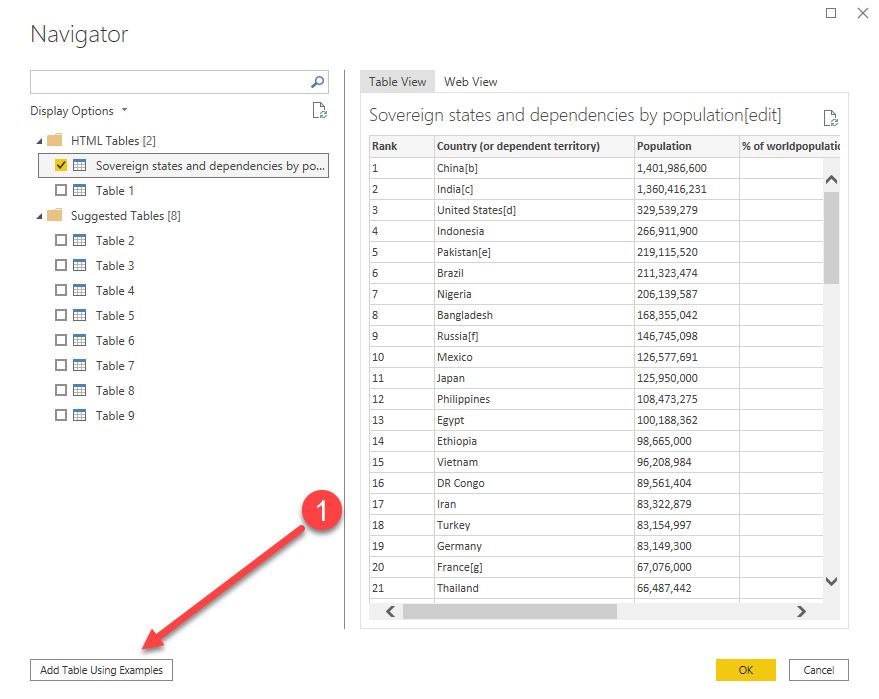
Create a new table by selecting the data source “Web” and paste the url of the page that you want to scrap.
The new screen will already parse your page and extract all the potential tables. Select the first one but click on “using examples”
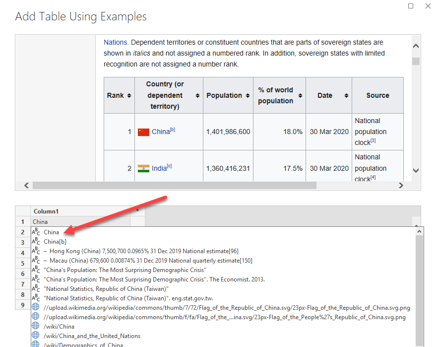
Another screen appears and ask you to provide examples. As soon as you’ll be starting to write the first letter of China, a pop-up will appear and will provide suggestion. select the one matching with your expectations.
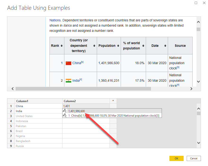
One example is rarely enough, you’ll probably have to provide a second (and potentially a third) example. Then the Ai engine will understand your examples and provide the results for the whole column. You can do the exact same thing for the second column.
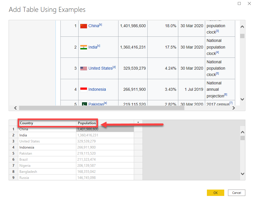
Then don’t forget to rename your columns with the expected names and click on OK. The table will be created with the expected values for the countries and population.
After this, you’ll surely have to sprinkle a bit of black magic to merge this information with other informations from John Hopkins University but it’s just business as usual. If you want to know more about this, just open the code on my GitHub account for the COVID-19 analysis.
This blog post is the second of a series related to parsing time series about COVID-19, you can find the first one here.
When dealing with time series, you should always check if your time series are event-based or cumulative. For a time series with a step of one day, an event-based time series will contain the count of events for a given day. A cumulative time series will contain the sum of the event of that day and of all the previous days! In this blog post I’ll explain how to transform a cumulative time series into an event-based.
As you can visualize in the picture above, the transformation is just consisting in taking the current element and substracting the previous.
We’ll create a function to handle this transformation. This function will expect a table with a column Date and another Value. The transformation will be executed on the column Value and the order will be determined by the column Date.
The first step is to sort the table by date and add an index.
let
    transformToIncremental = (source as table) =>
let
    indexedTable = Table.AddIndexColumn(
         Table.Sort(
             source
             ,{{"Date", Order.Ascending}}
         )
         , "Index", 0, 1
    )
    …
in
    normalizeTable
in
    transformToIncremental
Once the index added, you need to add a new column filled by application of the formula explained above.
addIncrement = Table.AddColumn(
    indexedTable
    , "Increment"
    , each try
               [Value] - indexedTable{[Index]-1}[Value]
           otherwise
               [Value]
    , type number
)
Once the column containing the expected value is there, we just need to select the two useful columns and don’t forget to rename the last one to match with the initial name.
The full code of this function is available here under:
let
    transformToIncremental = (source as table) =>
let
    indexedTable = Table.AddIndexColumn(Table.Sort(source,{{"Date", Order.Ascending}}), "Index", 0, 1)
    , addIncrement = Table.AddColumn(indexedTable, "Increment", each try [Value] - indexedTable{[Index]-1}[Value] otherwise [Value], type number)
    , normalizeTable = Table.RenameColumns(Table.SelectColumns(addIncrement, {"Date", "Increment"}),{{"Increment", "Value"}})
in
    normalizeTable
in
    transformToIncremental
If you follow the previous blog post, you’ll see that we can call this function from the function getTimeSeries. The idea is to execute the transformation for each time series … it means for each country. Based on this, we’ll start by grouping all the rows based on the GeographyKey. Each group will contain the GeographyKey but also two additional tables. The first one will contain all the fields related to geography and the second the time series for the given country
The first table containing the rows with geographical information should only contains duplicates. When expanding it will be important to not do a cardinal product of this table with the time series. We can just select the first row of this table and expand it.
Today, I was fed up with official communication around COVID-19 in Belgium. Media and officials are continuously reporting absolute figures: 71 deaths during the last 24 hours in Belgium and in the meantime 292 deaths in France. If you are not familiar with demography, you could think that the situation is worse in France than in Belgium … but as soon as you check a geography atlas and you find out that France has six times more inhabitants than Belgium, you change your mind.
I decided to use my skills with Power Query to wrap the figures of COVID-19. First step, get the raw data. Since a few days, a few scientists complain about the lack of raw data for Belgium, so I directly switched to an international source and opted for John Hopkins University dataset. For the population by country, I’d go for Wikipedia, on this page about the list of countries and dependencies by population.
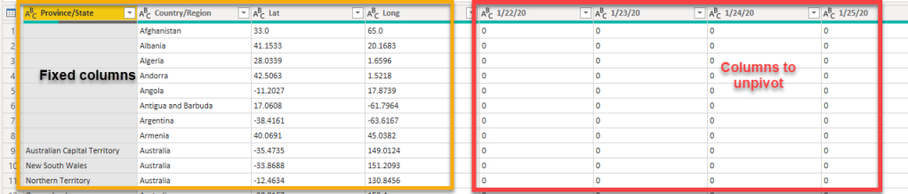
John Hopkins University is curating the figures from all over the world and provides three datasets. Each of them respectively contains figures about deaths, recovered and confirmed cases. In fact, each file is a matrix with on one axis the countries and on the second axis the dates. The three files are mostly identical.
Based on that information, I immediately took the decision to create a function that I’ll call for the three files. Why? Just to avoid to repeat myself three times. At a first glance, it could be seen as overengineering but when you have to maintain this, it’s a time saver! Only one place where you need to fix or perform some evolutions. Just imagine that tomorrow figures about hospitalizations were available … no need to copy/paste, just to call the function. The general design of the function is the following:
download the file and parse it as a CSV file
unpivot the date columns
parse the date
add some keys
switch from cumulative figures to day by day figures
Fix types for some columns
In this first blog post, I’ll cover all the steps except the fifth that will deserve its own blog post. In a third post, I’ll explain how to add figures about population by country to this dataset.
Let’s start by the skeleton of a function. The function will be expected the name of the dataset (deaths, confirmed or recovered).
let
    getTimeSeries = (name as text) =>
let
    …
in
    …
in
    getTimeSeries
To download a file hosted on GitHub, you need to use the raw version. The url is starting by raw.githubusercontent.com To compile the full url, I’ll do some concatenation of text values, usually easier when performed with the help of Text.Combine.
Once the file downloaded, you can open it as a CSV file. If you generated this step with the UI, pay attention that it will include an additional parameters with the count of columns (Columns). Based on file specifications (columns represents the dates), this count will change everyday. Just the remove this parameter, it’s not useful in that case. If you forget this parameter be aware that the downloaded file will be truncated to the count f columns specified in this parameter … will be embarassing to not have the last dates.
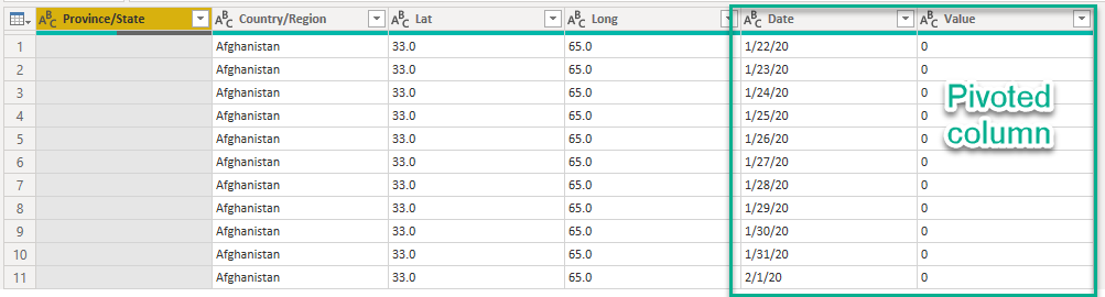
As we don’t know how many columns need to be unpivoted, we’ll use the function Table.UnpivotOtherColumns. This native function translates all columns other than a specified set into attribute-value pairs, combined with the rest of the values in each row. We’ll name this pair of columns Date and Value
The next challenge is to fix the format for dates. I’ll never understand why Americans are not opting for an international format. The format is the ugly M/D/YY. Power Query has some native functions to parse dates in uncommon format to the standard but it usually takes too much time to find the correct settings to achieve this. I’ll use a manual parsing to transform to the format YYYY-M-D. From that I know for sure that a type transformation will be supported. Let’s start by adding “20” in front of the transformation to write down the second twenty-one century. Then append the digits after the second “/”. Follow this by the digit(s) before the first “/” and then the digit(s) between the slash. Hopefully, Power Query has a set of native functions to help for this parsing with: Text.AfterDelimiter, Text.BeforeDelimiter and Text.BetweenDelimiters.
typedTable = Table.TransformColumnTypes(
   parseableDate
   ,{{"Date", type date}, {"Value", Int64.Type}}
)
I’ll add a column with the type of information that is contained in this file. Why? So I’ll ba able to merge the three files to create a huge table. Another approach would have been to create a fact table with three columns (one by file).
addInfoType = Table.AddColumn(
   typedTable
   , "InfoType"
   , each Text.Proper(name)
   , type text
)
You’ll notice that some countries (Canada, Australia, China, United Kingdom, France, Netherlands and Denmark) appear several times in the files. These countries have the details by province/state. When we’ll create our dimension geography, we’ll be in need to use a single field as key. Let’s build with a straightforward concatenation.
We’ll improve the function in the second blog post. But we can already take a look to the results of this function by creating three calls to this function each of them with the parameters deaths, recovered and confirmed. Here is an example of this call.
I’m currently working on the setup of a data quality dashboard and Power BI was our natural choice to display valuable information. For an advanced use-case, we needed to consume CSV files containing all the rows not validating a given data quality rule (violations). Each CSV file was completely different because each rule is consuming different information during the run. It means that in one file I could be facing the column EmployeeId and BirthDate but in the next file I could find a PublishDate and Area followed by Value. In the case of a specific project, all the data quality rules report a field related to a date information. The idea of the report was to count the violations by this date. Unfortunately, we quickly found a few issues with our CSV files:
Most of the time the column containing the date was named “DateTime” but it was not always the case
In some files, the first row (containing the header and so the columns’ name) was empty
In some files, the transformation from a JSON structure to a CSV was not correctly handled by the parser and we have the following information in place of the expected date: "value": "2018-01-01". The expected date is there but we need some additional parsing to extract it.
At the beginning, some of us thought that it would be easy to fix these issues by returning to the data quality team and ask them to fix these issues but it was not so easy. Identifing the rules needing a fix would be huge task (the CSV files are not created if the test is successful, maling it impossible to address this issue in one run and other impediments). I took the decision to go over this issue with the implementation of the following heuristic:
if the CSV has a column DateTime then we’ll use it
if the header is empty or no column is named DateTime then use the first column
if the content of the selected column is not a date then try to parse it as the inner content of a JSON element.
To implement this parsing, I started by the list of files and the table created from the CSV. In this list I’ll add a new column corresponding to the list of DateTime found in the CSV file applying the previously described heuristics. To implement theses heuristics, I created a function expecting one parameter, the original table retrieved when opening the CSV file.
let
    getDateTimes = (rawTable as table) =>
let
   …
in
   …
in
   getDateTimes
The first step is to promote the first row as the header containing all the column names.
We’ll consume this inline function to determine which column, we’ll need to keep. If this column exists then we’ll use it else we’ll use the first column.
targetColumn = if hasDateTimeColumn
    then {"DateTime"}
    else {List.First(Table.ColumnNames(csvTable))}
Now that we’ve identified the column, we can just keep this column and remove unneeded columns.
Unfortunatelly, we cannot be sure of the name of this column and it’s easier if we can correctly named it. We’ll renamed the first column with the expected name.
Now, we’ll need to get the value from this field. It could directly be the value or it could be a subpart of the a JSON element. To handle the different paths to obtain this value we’ll need to create a new internal function named getDateTime. Each row of the table will have to call this function to get its corresponding value. We can achieve this with the help of the native function Table.TransformColumns
The code of the function getDateTime is simply applying a trial and error. We first try to parse the value as a date. If it doesn’t work, we’ll consider to format the value in a JSON element and then extract the inner value. We can jump from the first path to the second simply with a try … otherwise ... structure.
Once, we’ve extracted the value, we can cast it as a date. That will enable us to check if our heuristic was correct or not beacuse at the end we’re expecting to get a date!
typedDateTimeTable = Table.TransformColumnTypes(
    parseDateTimes
    , {{"DateTime", type datetime}}
)
Finally, we just need to return the column DateTime.
typedDateTimeTable[DateTime]
When I explained to the team in charge of Power BI that we would not fix the issues at the root cause and that they’ll have to provide the data, they told me it was impossible. Sometimes, I believe in as many as 6 impossible things before breakfast! Eventually, it took me around 30 minutes to write this code on a bed in an hotel room. The heuristics were covering 99% of the cases. At contrario, solving the respective issues in the data quality tool and in the parsers would have taken many days (but will be done … later).
The full code:
let
    getDateTimes = (rawTable as table) =>
let
    csvTable = Table.PromoteHeaders(rawTable, [PromoteAllScalars=true])
    , hasDateTimeColumn = List.Contains(Table.ColumnNames(csvTable), "DateTime")
    , targetColumn = if hasDateTimeColumn then {"DateTime"} else {List.First(Table.ColumnNames(csvTable))}
    , rawDateTimeTable = Table.SelectColumns(csvTable, targetColumn)
    , renamedDateTimeTable = Table.RenameColumns(rawDateTimeTable, {{List.First(targetColumn), "DateTime"}})
    , parseDateTimes = Table.TransformColumns(renamedDateTimeTable, {"DateTime", getDateTime})
    , typedDateTimeTable = Table.TransformColumnTypes(parseDateTimes, {{"DateTime", type datetime}})
    , getDateTime = (value) =>
        let
            datePath = DateTime.From(value)
            , jsonPath = Json.Document(Text.Combine({"{", value, "}"}))[value]
        in
            try datePath otherwise jsonPath
in
    typedDateTimeTable[DateTime]
in
    getDateTimes
In a recent project, I was facing a really weird JSON structure. Each element of the JSON was more or less a dictionary with sparse keys. It means that the field names were different from an element to the other and that I was not really interested by the field name but more by the value of this field, independently of the field name.
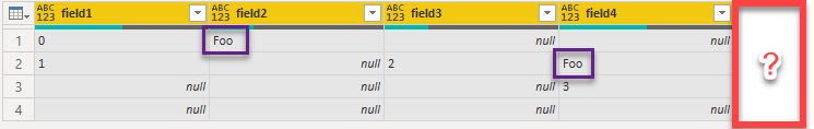
The structure of the JSON was the following: an array, with anonymous elements having different fields.
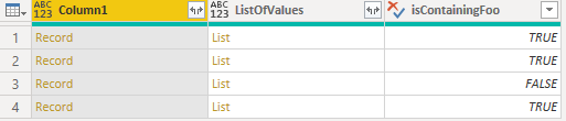
From this JSON, I needed to filter out all the elements without at least one of the value of any field set to “Foo”. From the previous example, it means that the third element should have been discarded (no “Foo” value).
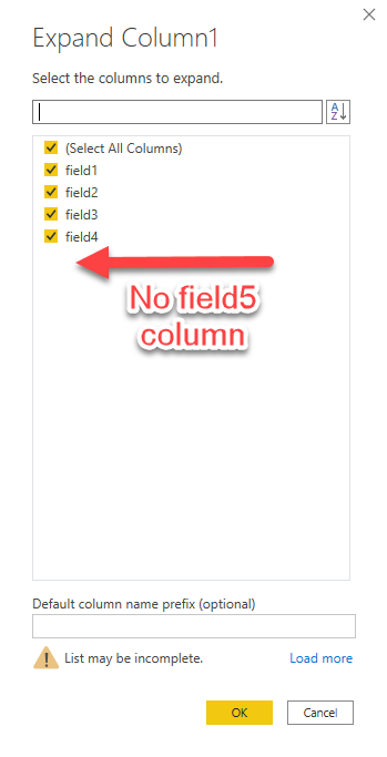
When facing JSON files, most of the time, we transform the list of records to a table and expand the records. Using the UI, it will generate the following code:
The first issue that we can immediately spot, is the lack of field5 in my final table. Indeed the UI doesn’t check the fourth element and don’t propose this field during the expand operation.
I could use it by hand, but in my case the name of the fields was completely random from one record to the other and I could not enlist all of them. even if I could overcome this issue, it will still be complex to iterate over all the columns and check the available values!
We definitively need another approach to solve this. In fact, we can use the dynamic structure of the record at our advantage, no need to expand it and transform the record into a static structure.
Using the function Record.FieldValues we can extract all the values from the different fields of the record. We’ll add this of values as a new column next to the record.
, addListOfValues = Table.AddColumn(
    tableFromSource
    , "ListOfValues", each Record.FieldValues([Column1])
)
Once we’ve this list of values, it’s straightforward to check if the value “Foo” is contained in this list, we just need to use the function List.Contains.
, addContainsFoo = Table.AddColumn(
    addListOfValues
    , "isContainingFoo"
    , each List.Contains([ListOfValues], "Foo")
    , type logical
)
We just have to filter on our new column to discard all the elements without a Foo value.
The full code is available here under:
let
   source = Json.Document(File.Contents("C:\Users\cedri\Desktop\sample.json")),
   tableFromSource = Table.FromList(source, Splitter.SplitByNothing(), null, null, ExtraValues.Error),
   addListOfValues = Table.AddColumn(tableFromSource, "ListOfValues", each Record.FieldValues([Column1])),
   addContainsFoo = Table.AddColumn(addListOfValues, "isContainingFoo", each List.Contains([ListOfValues], "Foo"), type logical),
   filteredRows = Table.SelectRows(addContainsFoo, each ([isContainingFoo] = true))
in
   filteredRows
For a solution I’m currently working on, I needed to get a list of all the tables of my solution with some information (name, position and type) of their respective columns. The goal was to execute this task on the Power BI Desktop application and pushing the dataset to the service was not an option.
To reach this goal, we’ll need to use a methodology known as reflection (or introspection) where the code is reading and parsing itself.
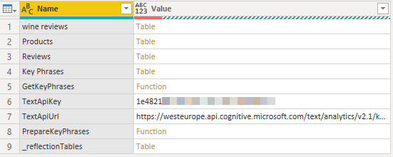
The first step is to list all the tables of my solution. To execute this step, I’ll use the keyword #sections. This keyword is from the same family than #shared but in place of returning all the native functions and the solution-specific tables, constants and functions, it will return all the sections. A section is equivalent to a namespace in .Net or Java, it’s a kind of container where content (functions, tables, constants) is uniquely named. In the current implementation of Power Query/M language, the content that you’re creating is always placed in the namespace Section1. This navigation is returning a list of records that we’ll turn into a table for easiness.
source = Record.ToTable(#sections[Section1])
As visible in the above screenshot, usage of this function returns the different constants, tables and functions written in my solution. In our case we just need to limit our scope to the tables. We can filter the content of my table based on the type of the value contained in my second column. To achieve this the function Value.Is combined with the token type table is the right choice. I’ll also remove all objects for which the name is starting by an underscore to avoid to work on this table created by this script.
holdTables = Table.SelectRows(
    source
    , each (
        Value.Is([Value], type table) and not Text.StartsWith([Name], "_")
    )
)
To get the list of columns and some information about them, we can use the function Table.Schema. In our case we’re only interested by the column name, position and type and we’ll limit the expansion to these cases.
The next step is to perform a bit of clean-up by removing some columns and typing remaining columns. Then, we can sort the table by table name and then by column position.
When developing an application relying on Azure Cosmos DB as the data backend, it’s always interesting to develop and run automated tests to check the integration between the business logic layer and the data layer. Nevertheless, creating a specific database and host it on azure.com, is an expensive and not so flexible solution. Hopefully, Microsoft is providing the Azure Cosmos DB Emulator to develop and test application interacting with Azure cosmos DB. To run our automated tests during the continuous build process, we can leverage this Emulator. As often, I’ll demonstrate the how-to with the Ci/CD service AppVeyor but this should be applicable to other CI/CD (on-premises or cloud-based).
The good news with AppVeyor is that a recent version of the Azure Cosmos DB Emulator is already provided in the build image. We don’t need to install it before anything. If you really want the last version of this emulator or if you’re using another CI/CD service, I’ll explain at the end of this blog post how to download and install the emulator (and also how to uninstall it).
The first step is to start the emulator. The emulator is located on C:\Program Files\Azure cosmos Db Emulator\CosmosDb.Emulator.exe and this executable is expecting arguments to define the action to execute. By default, without argument, you’ll just start the exe. In this case, we need to ask the emulator to start without displaying UI information and we can also ask it to not start the Data Explorer (that is dedicated to UI interactions that anyway we won’t be able to use during a build). The two arguments to pass to the exe are: /NoUI /NoExplorer.
By default in v2.7, the explorer is just enabling the SQL API. If you want to use other API such as Cassandra, Gremlin or MongoDB then you’ll have to enable the endpoints. In this case, we’ll enable the Gremlin endpoint by providing the argument /EnableGremlinEndpoint. It’s also possible to define on which port the emulator will be listening for this endpoint but I usually don’t change them. If you want to get an overview of all the flags that you can activate or disable in the emulator just check on your own computer by submitting the command CosmosDb.Emulator.exe /help.
To start the emulator with the default endpoint for Gremlin in the context of a CI/CD service, the final command is:
"C:\Program Files\Azure Cosmos DB Emulator\CosmosDB.Emulator.exe" /NoExplorer /NoUI /EnableGremlinEndpoint
You can place this command in a batch file named start-emulator.cmd
If you just submit this command in the install step of your CI/CD workflow, you’ll have to face difficult times. Indeed, the Emulator is just running and listening on ports, so this command is never ending. On a CI/CD build, it means that the command will run on the main process of the CI/CD build and block everything, eventually your build will hang out. To avoid this, you’ll need to execute this command in another process. With PowerShell, you can just do this with the cmdlet Start-Process "start-emulator.cmd".
The emulator always take a few seconds to fully start. It’s important to check that the port is open before effectively using it or you could have unexpected exceptions due to the unavailability of the emulator. To avoid this start the emulator as soon as possible (before your build) and use it as late as possible (run the tests relying on it as the last tests). Nevertheless, it’s always a good idea, to check if this tool is correctly running before using it. To perform this check, you can assess that the port is effectively listening. Following PowerShell script is doing the job by checking if it’s possible to connect to the port at regular interval as long as the port is not available. When the port is available, the script display a positive message and continue.
Now that the emulator is started, you’ll need to create a database and a collection. It’s important to note that even if you want to create a graph database (Gremlin) and the Gremlin API is listening on port 8901 (by default), you’ll have to connect to the SQL API at the port 8081 (by default) to create the database and the collection. This is valid for all the api kind and not just for Gremlin. In fact, if you want to manage your Azure Cosmos DB instance, you must connect to the SQL API.
To create a database and a collection (if they don’t exist), you’ll need the Microsoft.Azure.DocumentDB package. Once installed, you’ll be able to use the methods CreateDatabaseIfNotExistsAsync and CreateDocumentCollectionIfNotExistsAsync of the class DocumentClient. The response of these two methods returns information about what happened (the database/collection was already existing or has just been created).
using (var client = new DocumentClient(sqlApiEndpoint, authKey))
{
    var database = new Database() { Id = databaseId };
    var databaseResponse = client.CreateDatabaseIfNotExistsAsync(database).Result;
    switch (databaseResponse.StatusCode)
    {
        case System.Net.HttpStatusCode.OK:
            Console.WriteLine($"Database {databaseId} already exists.");
            break;
        case System.Net.HttpStatusCode.Created:
            Console.WriteLine($"Database {databaseId} created.");
            break;
        default:
            throw new ArgumentException($"Can't create database {databaseId}: {databaseResponse.StatusCode}");
    }

    var databaseUri = UriFactory.CreateDatabaseUri(databaseId);
    var collectionResponse = client.CreateDocumentCollectionIfNotExistsAsync(databaseUri, new DocumentCollection() { Id = collectionId }).Result;
    switch (collectionResponse.StatusCode)
    {
        case System.Net.HttpStatusCode.OK:
            Console.WriteLine($"Collection {collectionId} already exists.");
            break;
        case System.Net.HttpStatusCode.Created:
            Console.WriteLine($"Database {collectionId} created.");
            break;
        default:
            throw new ArgumentException($"Can't create database {collectionId}: {collectionResponse.StatusCode}");
    }
}
Once the database created, you’ll need to populate it before you can effectively run your tests on it. This is usually something that I code in the OneTimeSetUp of my test-suite. To proceed, you must create a few Gremlin commands to add vertices and edges such as:
Then you’ll have to execute them. Tiny reminder: don’t forget that you’ll have to use the Gremlin API endpoint and not anymore the SQL API endpoint! The driver to connect to this API is the Gremlin.Net driver available on nuget and the source code is available on GitHub on the repository of TinkerPop. Once again, the usage is relatively straightforward, you first create an instance of a GremlinServer and then instantiate a GremlinClient to connect to this server. Using the method SubmitAsync of the class GremlinClient, you’ll send your commands to the Azure Cosmos DB Emulator.
var gremlinServer = new GremlinServer(hostname, port, enableSsl, username, password);

using (var gremlinClient = new GremlinClient(gremlinServer, new GraphSON2Reader(), new GraphSON2Writer(), GremlinClient.GraphSON2MimeType))
{
    foreach (var statement in Statements)
    {
        var query = gremlinClient.SubmitAsync(statement);
        Console.WriteLine($"Setup database: { statement }");
        query.Wait();
    }
}
Now that your database is populated, you can freely connect to it and run your automated tests. Writting these test is another story (and another blog post)!
Back to the first step … as stated before I took the hypothesis that Azure Cosmos DB Emulator was already installed on your CI/CID image and that the version suited your needs. If it’s not the case, that’s not the end of the world, you can install it by yourself.
Before, you start to uninstall and install this software, it could be useful to check the version of the current installation. The following PowerShell script is just displaying this:
Write-Host "Version of ComosDB Emulator:" ([System.Diagnostics.FileVersionInfo]::GetVersionInfo("C:\Program Files\Azure Cosmos DB Emulator\CosmosDB.Emulator.exe").FileVersion)
If you need to install a new version of Azure Cosmos DB Emulator, the first action is to remove the existing instance of Azure Cosmos DB Emulator. If you don’t do it, the new installation will succeed but the emulator will never start correctly. The black magic to remove an installed software is to use the Windows Management Instrumentation Command-line. This command is surely not really fast but it’s doing the job.
wmic product where name="Azure Cosmos DB Emulator" call uninstall
Then, you can download the last version of Azure Cosmos DB Emulator at the following shortcut url: https://aka.ms/cosmosdb-emulator
You should now be able to install, start and populate your Azure cosmos DB Emulator on your favorite CI/CD server … just a few tests to write and you’ll have some end-to-end tests running with Azure Cosmos DB Emulator.
The following appveyor.yml statements should do the job:
install:
# Install the Azure CosmosDb Emaulator with the option /EnableGremlin
- wmic product where name="Azure Cosmos DB Emulator" call uninstall
- ps: Start-FileDownload 'https://aka.ms/cosmosdb-emulator' -FileName 'c:\projects\cosmos-db.msi'
- cmd: cmd /c start /wait msiexec /i "c:\projects\cosmos-db.msi" /qn /quiet /norestart /log install.log
- ps: Write-Host "Version of ComosDB Emulator:" ([System.Diagnostics.FileVersionInfo]::GetVersionInfo("C:\Program Files\Azure Cosmos DB Emulator\CosmosDB.Emulator.exe").FileVersion)
- ps: Start-Process "start-emulator.cmd"
Don’t forget to check/wait for the Emulator before executing your tests:
Until now, you’ve always returned the last step of our query. But it’s not always what we want! In the previous query, we’ve returned the karatekas having defeated the karatekas who defeated my daughter. One of the issue of this query was that we didn’t know who defeated who.
We can fix this problem by returning tuples containing the two karatekas corresponding to the vertices in green on this drawing.
To achieve this, we’ll need to give an alias to the selection performed at the third intermediate step (and also to the latest). Gremlin as an operator named as to give aliases.
The following query is just assigning aliases to the interesting steps:
At that moment, if you executed the query, the result would be identical to what it was previously. Just giving aliases is not enough, you’ll also have to instruct to Gremlin to make some usage of them. The simpler usage is to select them. This operation ensure that the aliased vertices are part of the result of the query.
It’s usually not suited to get the whole list of properties. Most of the time we’ll only be interested by a subset of the properties in this case the fullName. To project the vertices to a single property, we can use the operation by provided by Gremlin.
You’ll have to learn a few additional operations to traverse a graph. The first set of operations are inE and outE. These two operations let you select all the edges respectivelly ending and starting from the selected vertex. The example here under show the result (in green) of the operation outE for a given vertex.
The following query is returning all the edges having the label participates and starting from the vertex representing a given karateka.
The result of this query is a list of edges. From this result we can see that the starting node is always the given karateka and that each edge is linking to a bout.
The same kind of operations exist for selecting vertices being the end or the start of a selected edge. These functions are named outV and inV.
The following query is starting from a karateka, then jumping the the edges having the label participates and then jumping to all the vertices being the end of the previously selected edges.
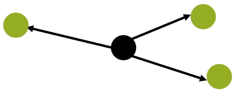
Most of the time, you don’t really want to select the edges. They are just a some means to go from one vertex to any adjacent vertex. for convenience, Gremlin is supporting two operations in and out. They are the equivalent of respectively outE followed by inV and inE followed by outV.
The following drawing explains that starting from the black vertex and using a in operation, you’ll directly select the three adjacent vertices.
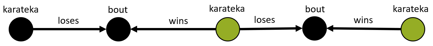
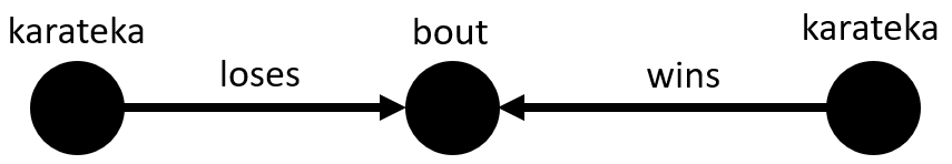
A good usage of the traversing of a graph will be to know the names of all the karateka having defeated a given karateka. To write this query we’ll first select the initial karateka, then going to all the bouts where the edge is labelled loses and corresponding to all the bouts where the karateka has been defeated. Having this list of bouts we just need to follow the edges labelled as wins to know the name of the winner.
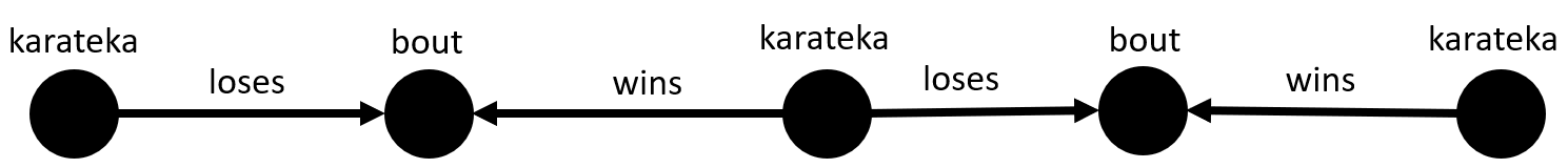
We can go a bit further and check if these karatekas have already been defeated by someone or not. To achieve this, I’ll apply the exact same pattern and use the edges loses and wins from the second karateka.
As you can see the first and last names but also the second and third are identical. The reason is that these two karatekas have defeated twice one of the three karatekas listed above (or once two of them). That’s really important to understand that Gremlin doesn’t automatically deduplicate the vertices. If you want to achieve this, just use the function dedup
Note that I applied the function dedup to the vertices and not to the property fullName. The reason is to avoid to consider as duplicates two karatekas that are just homonyms.
The next blog post will be about the step modulator … and how to return a result where the selected vertices are not the last vertices traversed by the query!
Properties are always attached to a vertex or an edge and give some information about this vertex or edge. Using Azure Cosmos DB, you’ll always have a property named pk that is mandatory and automatically generated by Azure Cosmos DB
      "pk": [
        {
          "id": "karateka.70|pk",
          "value": 1
        }
      ],
pk stands for partition key. Partition keys are an important feature of Azure Cosmos DB but I’ll explain them in a future dedicated post.
Other properties always have the same structure. The name of JSON field is the name of Gremlin property. Each JSON field contains an array of values for this property. Indeed, in Gremlin each property is multi-valued, we’ll come back to this later in this post. Each property’s value has an id having for value a GUID automatically attributed by the Azure Cosmos DB engine and a second field named value keeping track of the effective value of the property.
If you want to add a property to a vertex, you don’t need to perform any explicit change to the underlying schema. Graph databases are schema-less. It means that you can quickly add a new property by just specifying it. Naturally, it has some drawbacks and any typo could create a new property in place of editing an existing one.
To add a property to a vertex, you first need to select this vertex as explain in the previous blog post and then apply the operator property. This operation is expecting the property’s name and the property’s value as parameters:
It’s possible to add a property to more one than vertex. To achieve this, just select multiple vertices and define the common property. In the example below, I’m assigning the same birthday to my twin daughters.
As explained above, Gremlin natively support multi-valued properties. If you want to define a property having more than one property, you’ll have to specify it as the first parameter of the operator property by specifying the keyword list. The next query is adding a few middle names to a karateka.
This query is returning a really flat and compact JSOn document with just the values of the properties.
[
  "Charlier",
  "Alice"
]
When selecting multiple vertices this operator could be useless due to the fact that you don’t have the values grouped by vertex and that you don’t know the mapping between the property and the value. If you want a more explicit view on the property you can use the operator valueMap.
The result of this query will be an explicit JSON document, listing all the requested properties and grouping them by vertex. Once again if a property is not existing for a given vertex, it won’t be an issue.
It’s also possible to drop several properties on several vertices. If the properties are not existing it won’t create an exception once again a benefit of schema-less databases.